KumoRFM in Snowflake Notebooks#

This guide walks you through running KumoRFM inside Snowflake Notebooks. Your data never leaves Snowflake -you connect, build a graph, and make predictions all from within a notebook.

By the end of this guide you will:

Create a Snowflake Notebook and connect it to a compute pool
Install the Kumo SDK
Build a graph from your data (three ways to do this)
Run prediction queries using KumoRFM

Tip

Want to skip ahead? Download the example notebook and import it into Snowflake. It comes pre-filled with all the code from this guide -just update the settings and run the cells.

Setup#

Follow Steps 1–5 below to set up your notebook. These steps are the same regardless of which data source you use later.

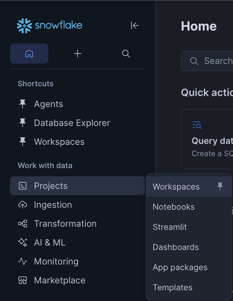
Step 1. Open Snowflake and go to Workspaces#

Snowflake sidebar showing Projects > Workspaces

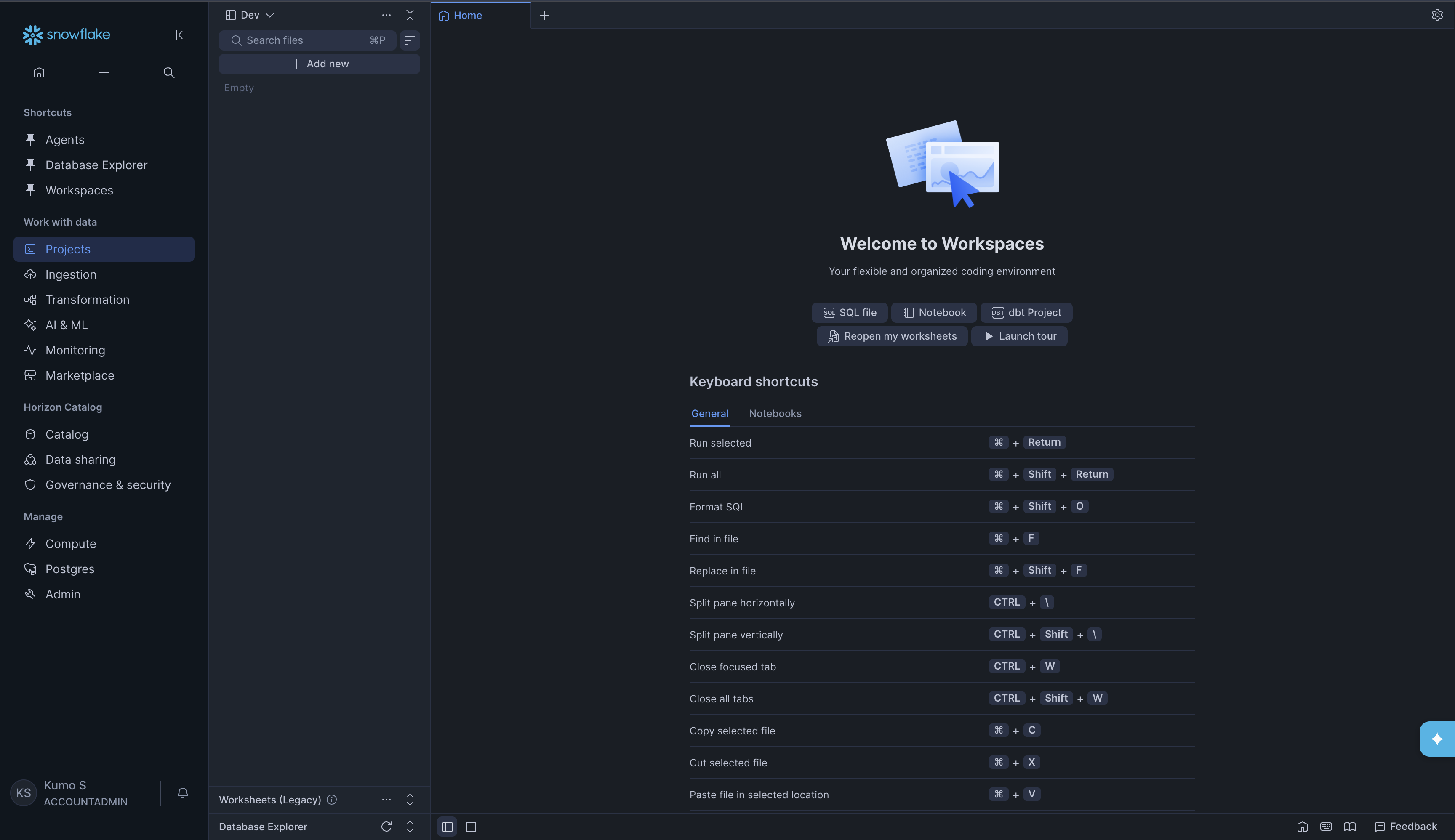
You will see the Welcome to Workspaces page with options to create SQL files, Notebooks, and dbt Projects.

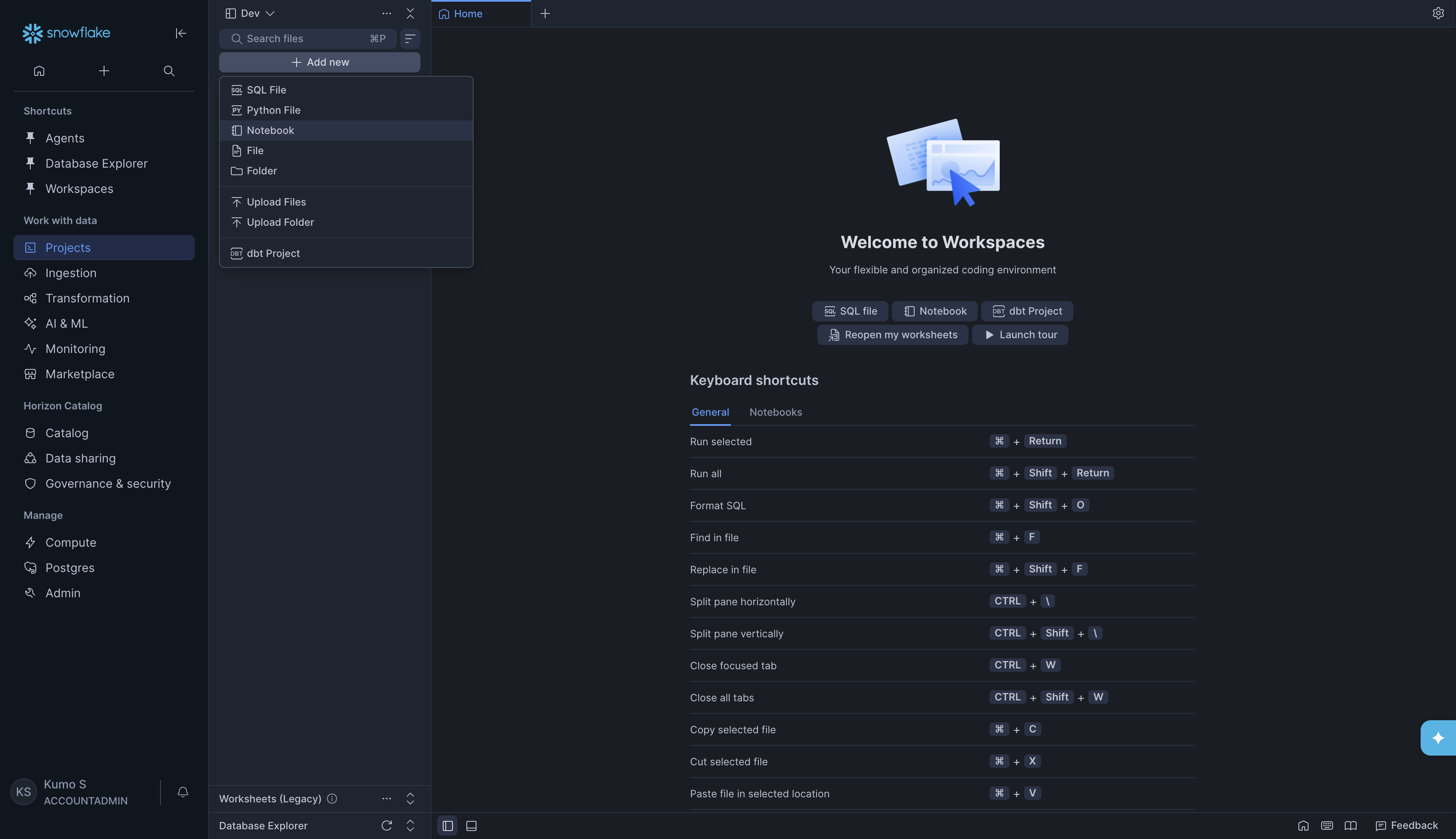
Step 2. Create a new Notebook#

In the left panel, click + Add new. A dropdown menu will appear. Click Notebook.

Add new dropdown showing Notebook option

A new empty notebook will open. You can rename it by clicking the title at the top (for example, RFM_DEMO.ipynb).

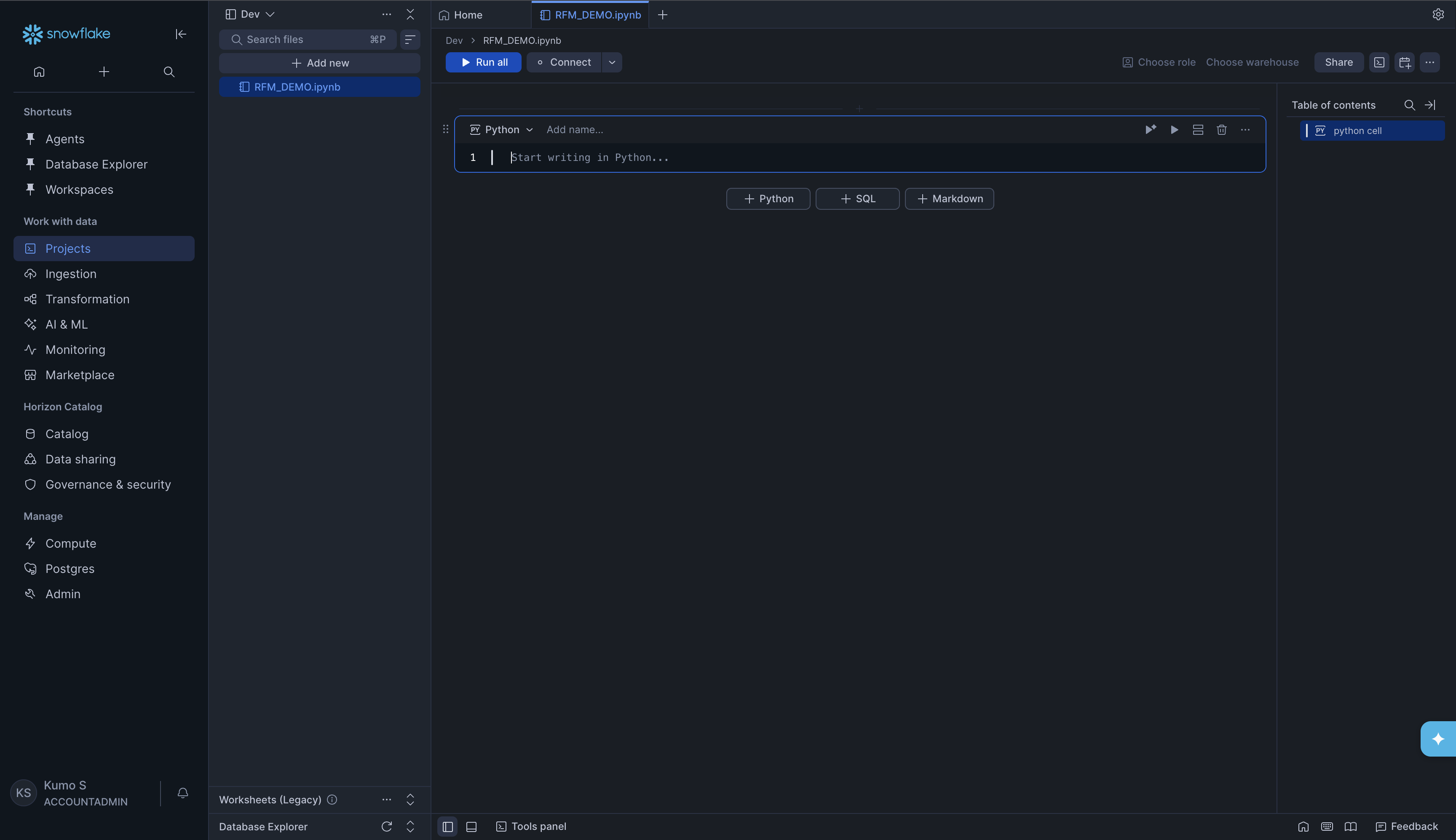
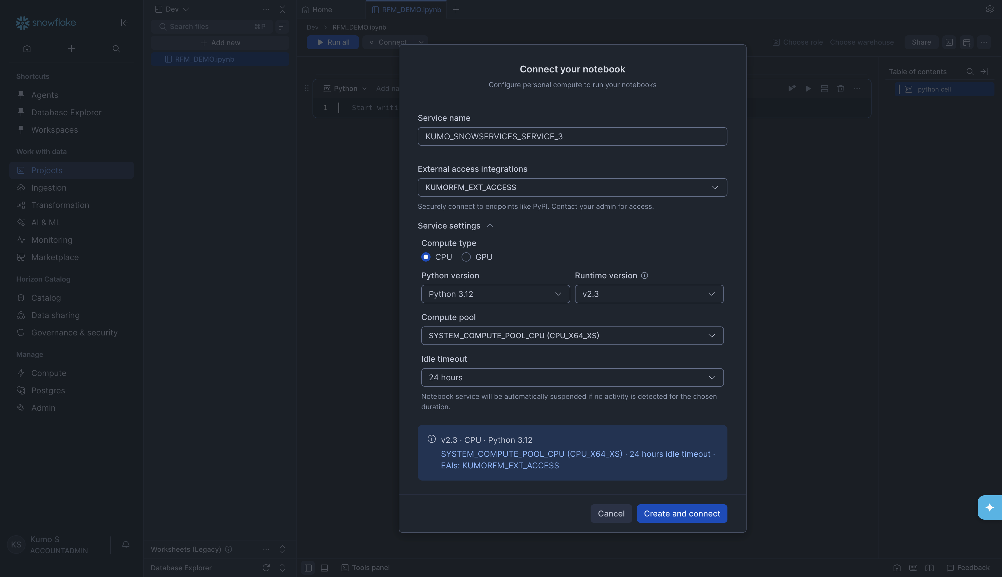
Step 3. Connect your Notebook#

Before you can run any code, you need to connect the notebook to a compute resource. Click the Connect button at the top of the notebook. A dialog called Connect your notebook will appear.

Fill in the following settings:

Setting	What to enter
Service name	A name for the notebook service (e.g., `KUMO_SNOWSERVICES_SERVICE_3`)
External access integrations	Select an external access integration that has internet access (e.g., one that allows connections to PyPI). This is needed to install packages. Contact your Snowflake admin if you do not have one set up.
Compute type	Select CPU
Python version	Select Python 3.12 (or the latest available)
Runtime version	Select v2.3 (or the latest available)
Compute pool	Select `SYSTEM_COMPUTE_POOL_CPU (CPU_X64_XS)` or another CPU pool available to you
Idle timeout	Choose how long the notebook stays running when idle (e.g., 24 hours)

Click Create and connect. Wait for the status indicator at the top of the notebook to turn green (showing Connected).

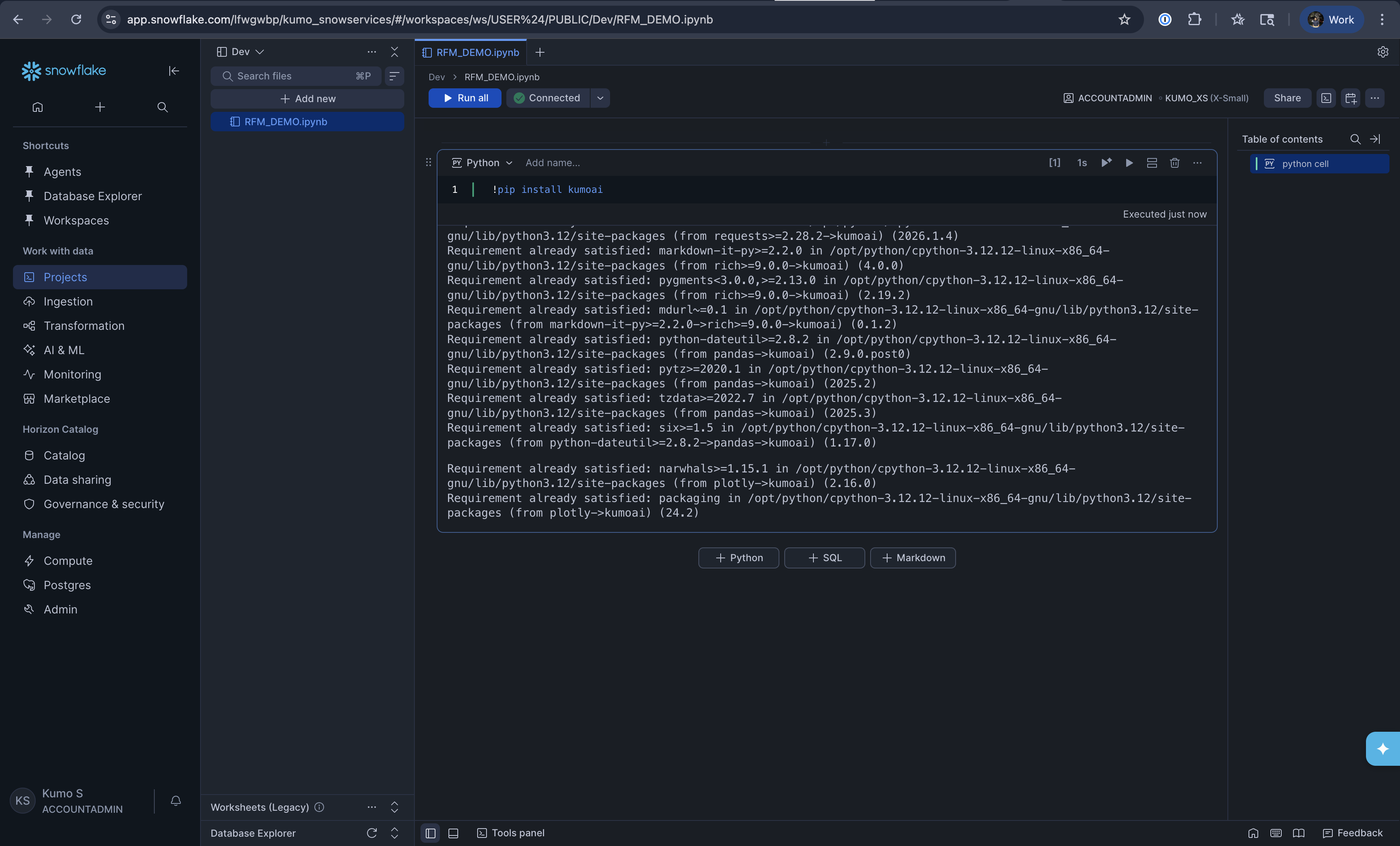
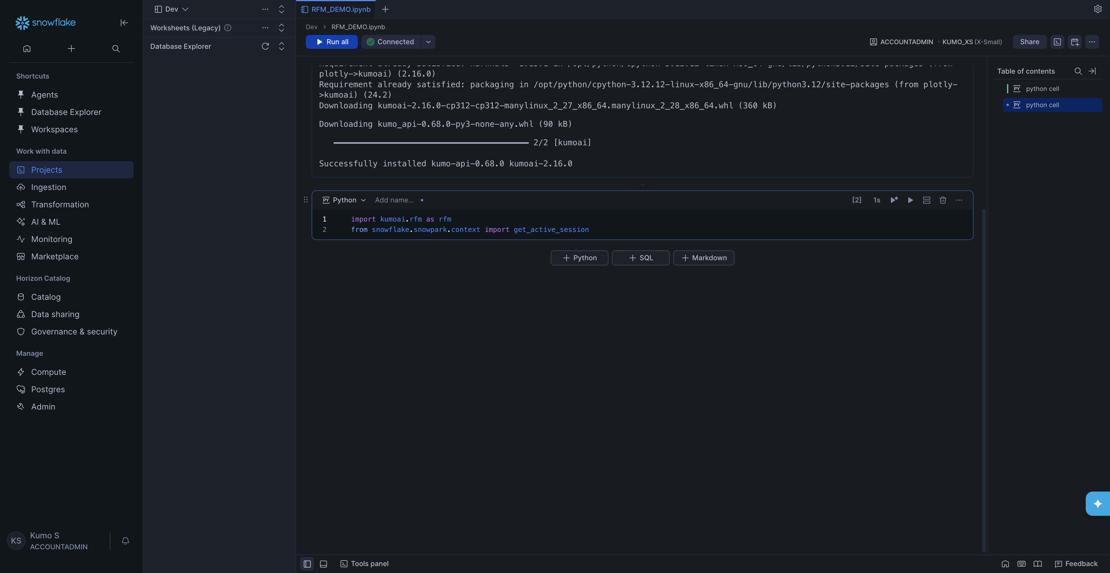
Step 4. Install the Kumo SDK#

In the first cell of your notebook, install the kumoai package by running:

!pip install kumoai

You will see pip output showing the package being installed along with its dependencies. Once it finishes, you are ready to use KumoRFM.

Step 5. Import and initialize#

In the next cell, import the required modules:

import kumoai.rfm as rfm
from snowflake.snowpark.context import get_active_session

In the next cell, get the Snowflake connection and initialize KumoRFM:

connection = get_active_session().connection
rfm.init()

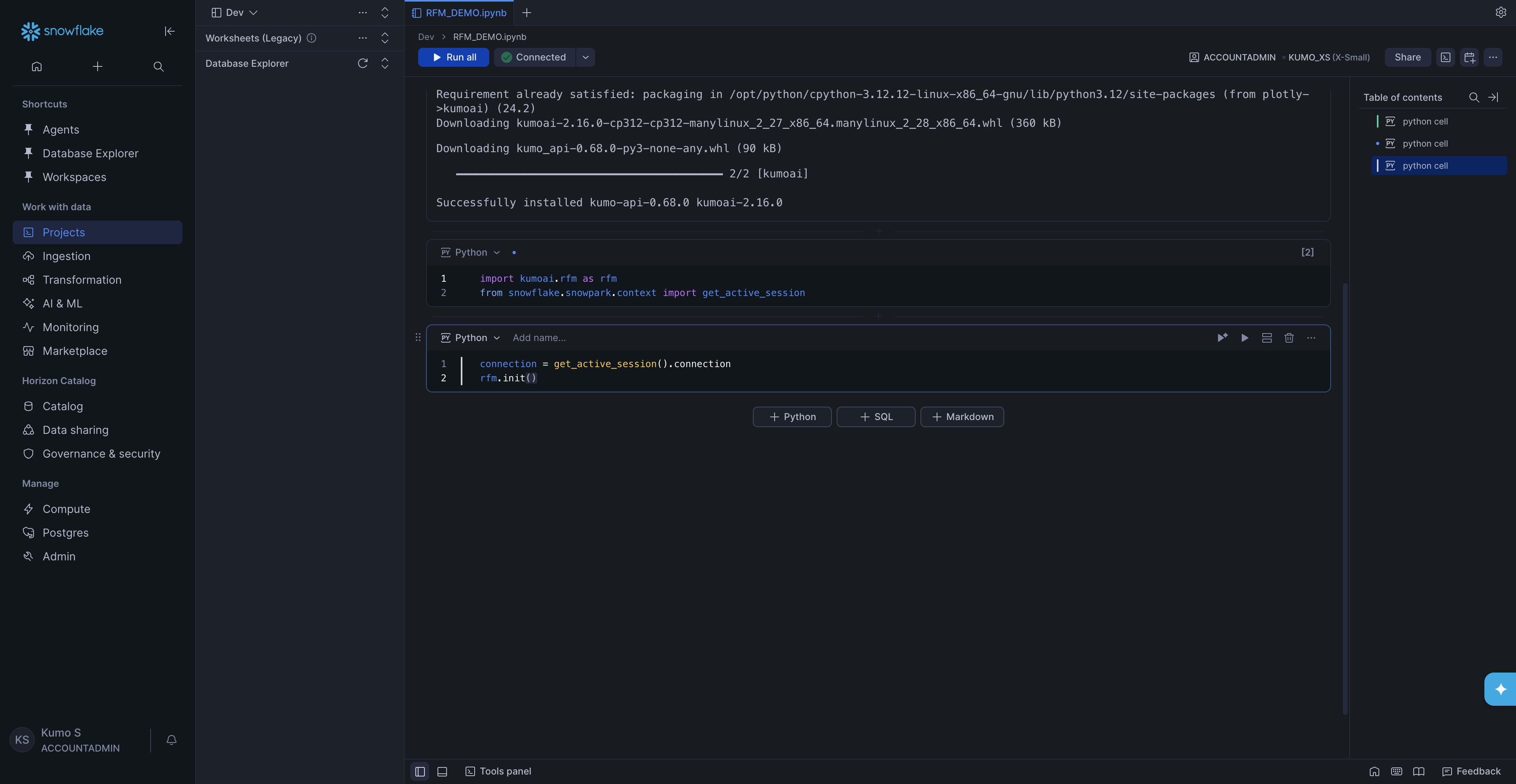
That’s it -KumoRFM is now ready to use. Next, pick one of the three options below to build a graph from your data.

Build Your Graph and Make Predictions#

A graph is a description of your data. It defines:

Your tables and their columns
The primary and foreign key relationships between tables
Semantic definitions on fields, such as whether a column is categorical

KumoRFM uses the graph to understand the structure of your data and answer prediction queries without training a model from scratch.

There are three ways to build a graph in Snowflake Notebooks. Pick the one that fits your situation:

Option A -From pandas DataFrames (quick testing with small datasets; the data must fit in notebook memory)
Option B -From a Snowflake Semantic View (recommended for production; scales to any data size and captures rich semantic definitions)
Option C -From Snowflake tables with manual table selection (no semantic view required; scales to any data size)

Note

Option A loads your tables into pandas DataFrames inside the notebook, so the notebook’s compute pool needs enough memory to hold the data. For large datasets, use Option B or Option C instead, which read data directly from Snowflake without loading it into memory.

All three options end the same way: you initialize KumoRFM with rfm.KumoRFM(graph) and run predictions with model.predict(query).

Option A: From pandas DataFrames (LocalGraph)#

This is the easiest way to get started. You load data into pandas DataFrames (from S3, local files, or anywhere else) and let KumoRFM build a graph from them.

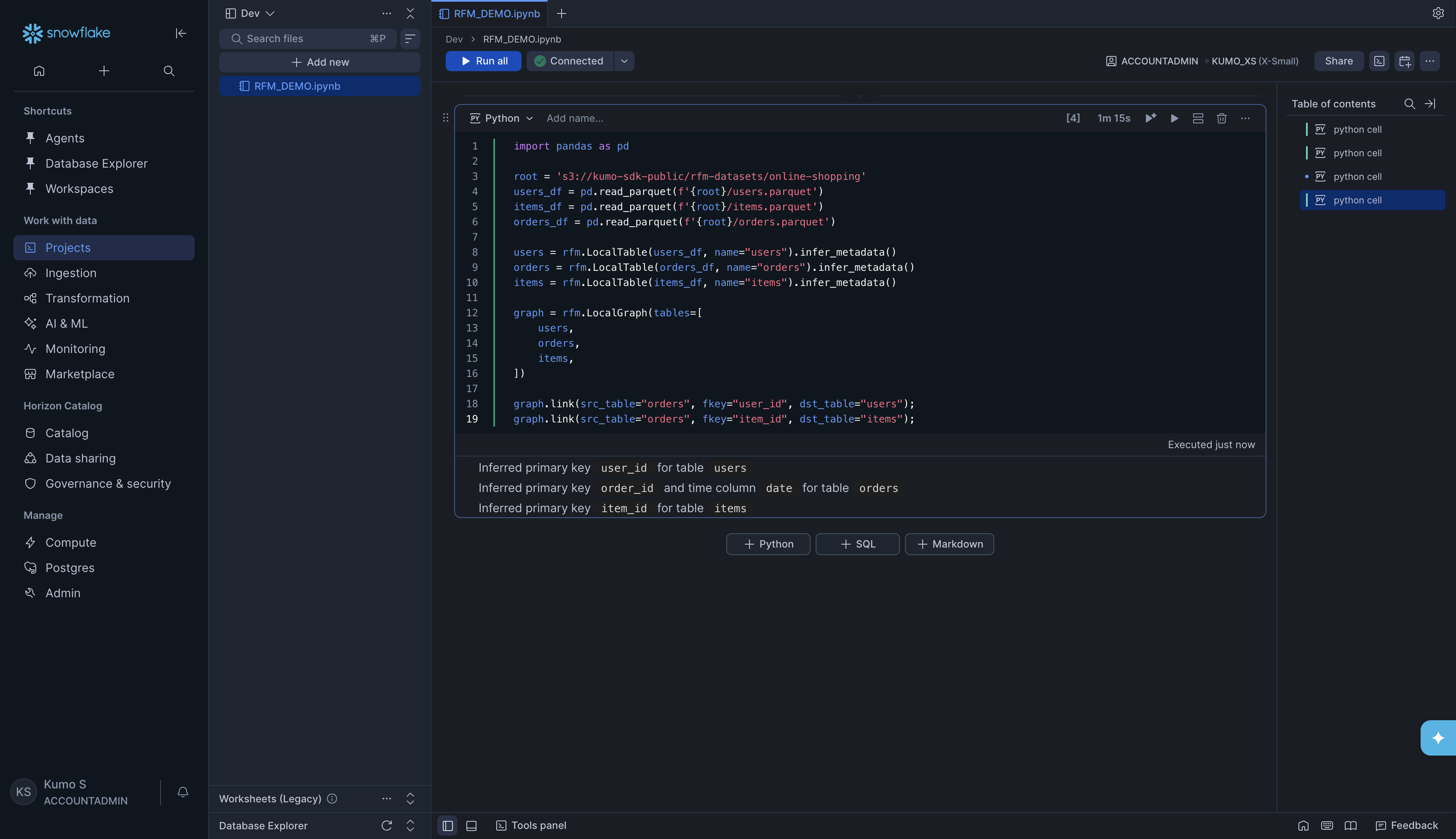
Load the data and create tables:

import pandas as pd

root = 's3://kumo-sdk-public/rfm-datasets/online-shopping'
users_df = pd.read_parquet(f'{root}/users.parquet')
items_df = pd.read_parquet(f'{root}/items.parquet')
orders_df = pd.read_parquet(f'{root}/orders.parquet')

users = rfm.LocalTable(users_df, name="users").infer_metadata()
orders = rfm.LocalTable(orders_df, name="orders").infer_metadata()
items = rfm.LocalTable(items_df, name="items").infer_metadata()

graph = rfm.LocalGraph(tables=[
    users,
    orders,
    items,
])

graph.link(src_table="orders", fkey="user_id", dst_table="users");
graph.link(src_table="orders", fkey="item_id", dst_table="items");

KumoRFM will automatically detect primary keys and time columns from your data. You will see output like:

Inferred primary key  user_id  for table  users
Inferred primary key  order_id  and time column  date  for table  orders
Inferred primary key  item_id  for table  items

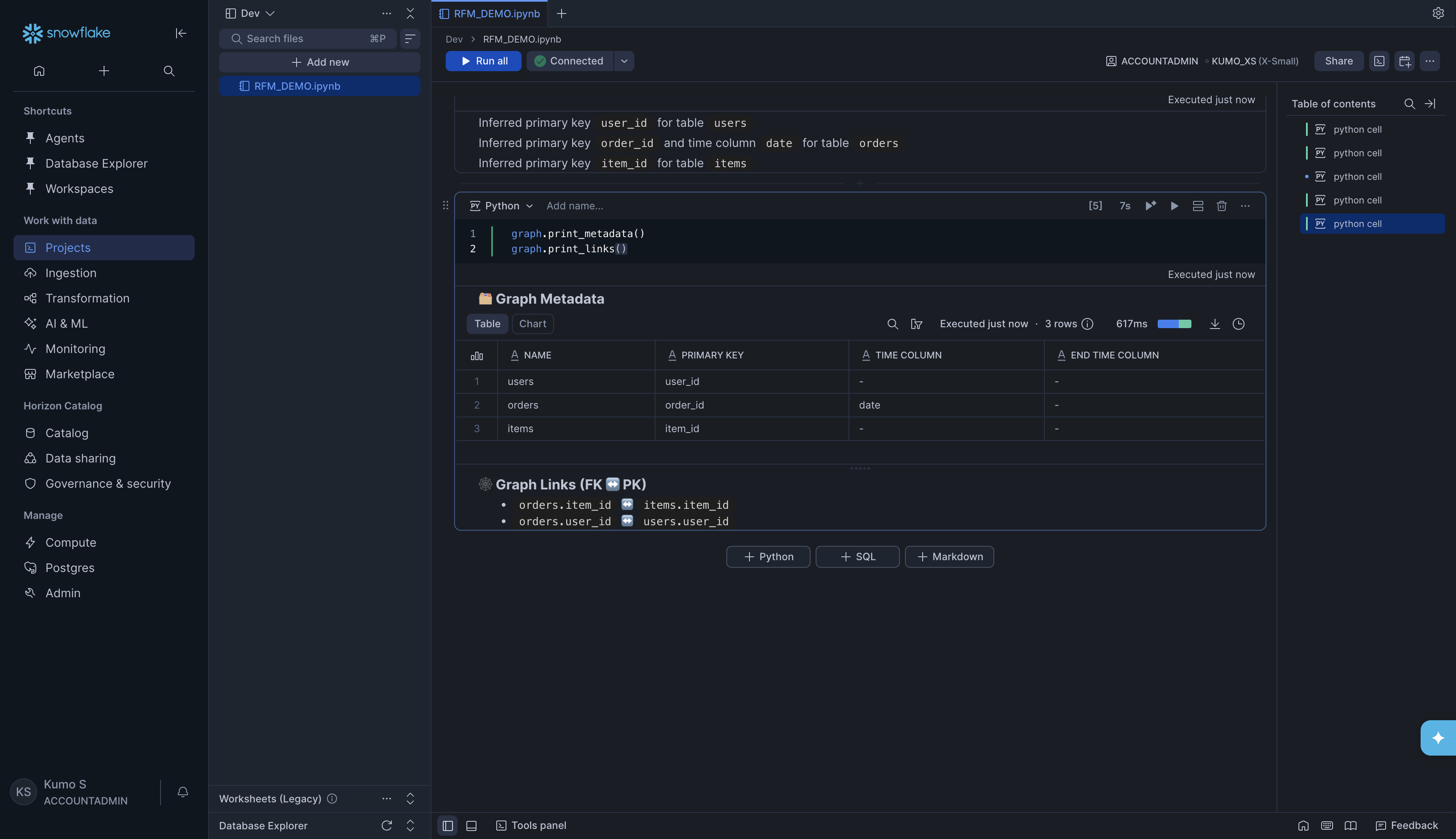
Inspect the graph (optional but recommended):

graph.print_metadata()
graph.print_links()

This shows a table of all your tables with their primary keys and time columns, plus a list of all the links (foreign key relationships) between them.

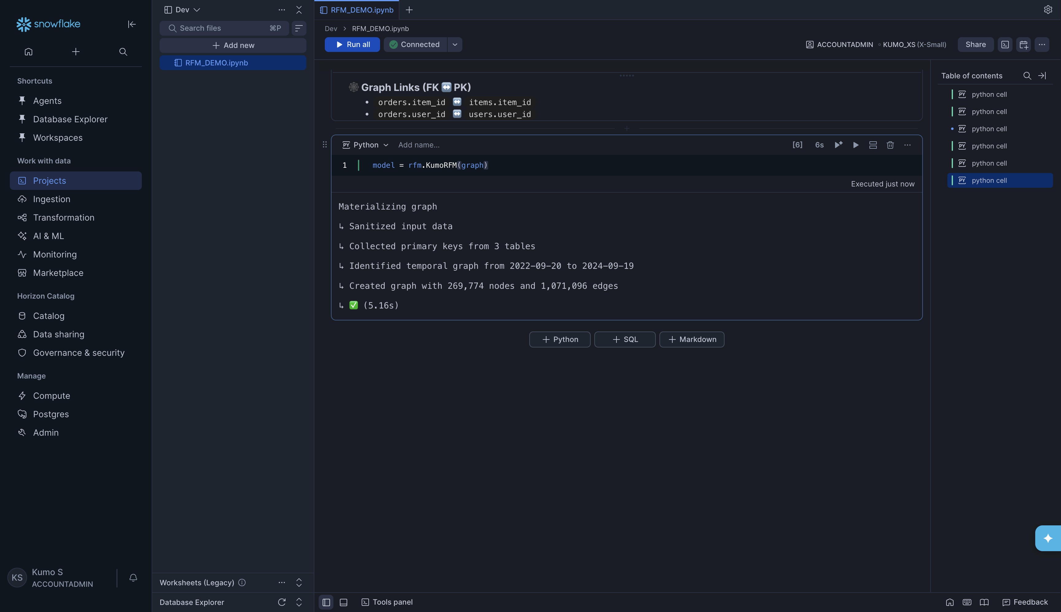
Load the graph into KumoRFM:

model = rfm.KumoRFM(graph)

You will see progress output like:

Materializing graph
↳ Sanitized input data
↳ Collected primary keys from 3 tables
↳ Identified temporal graph from 2022-09-20 to 2024-09-19
↳ Created graph with 269,774 nodes and 1,071,096 edges
↳ ✅ (5.16s)

Make a prediction:

Now you can write a Predictive Query (PQL) and get results. For example, to predict whether users 42 and 123 will make zero orders in the next 90 days (customer churn):

query = "PREDICT COUNT(orders.*, 0, 90, days)=0 FOR users.user_id IN (42, 123)"

df = model.predict(query)
display(df)

KumoRFM will show progress and return a DataFrame with predictions:

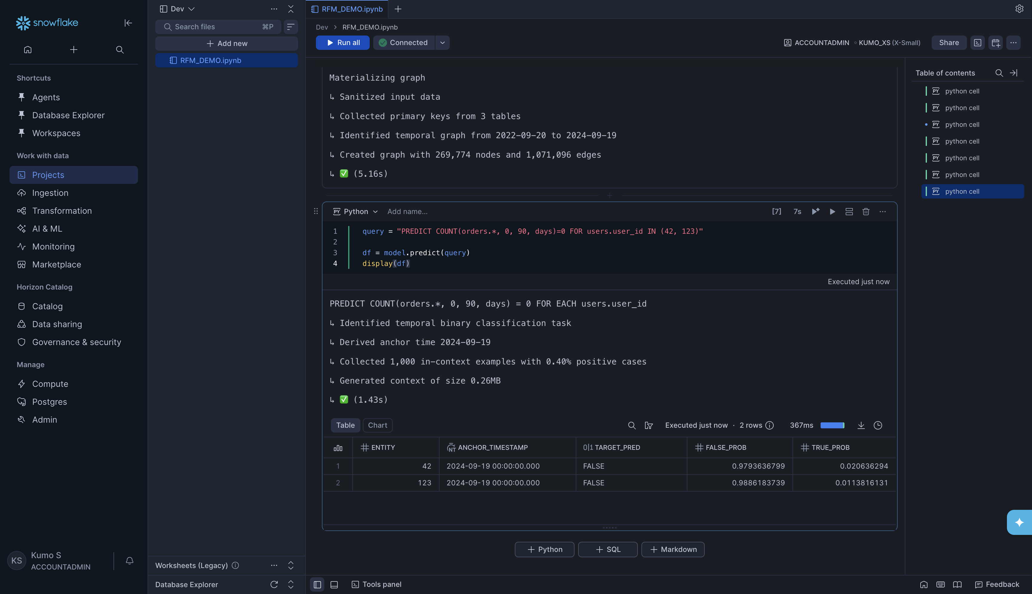
The result tells you:

ENTITY -The user you predicted for
ANCHOR_TIMESTAMP -The point in time the prediction is made from
TARGET_PRED -The predicted class (TRUE = will churn, FALSE = will not churn)
FALSE_PROB / TRUE_PROB -The probability of each outcome

Option B: From a Snowflake Semantic View#

If your organization has a Snowflake Semantic View set up, you can build a graph directly from it. The semantic view already contains table definitions and relationships, so KumoRFM reads everything automatically.

Set the database (if needed). Add a SQL cell and run:

USE DATABASE NL2PQL_TESTING_V0

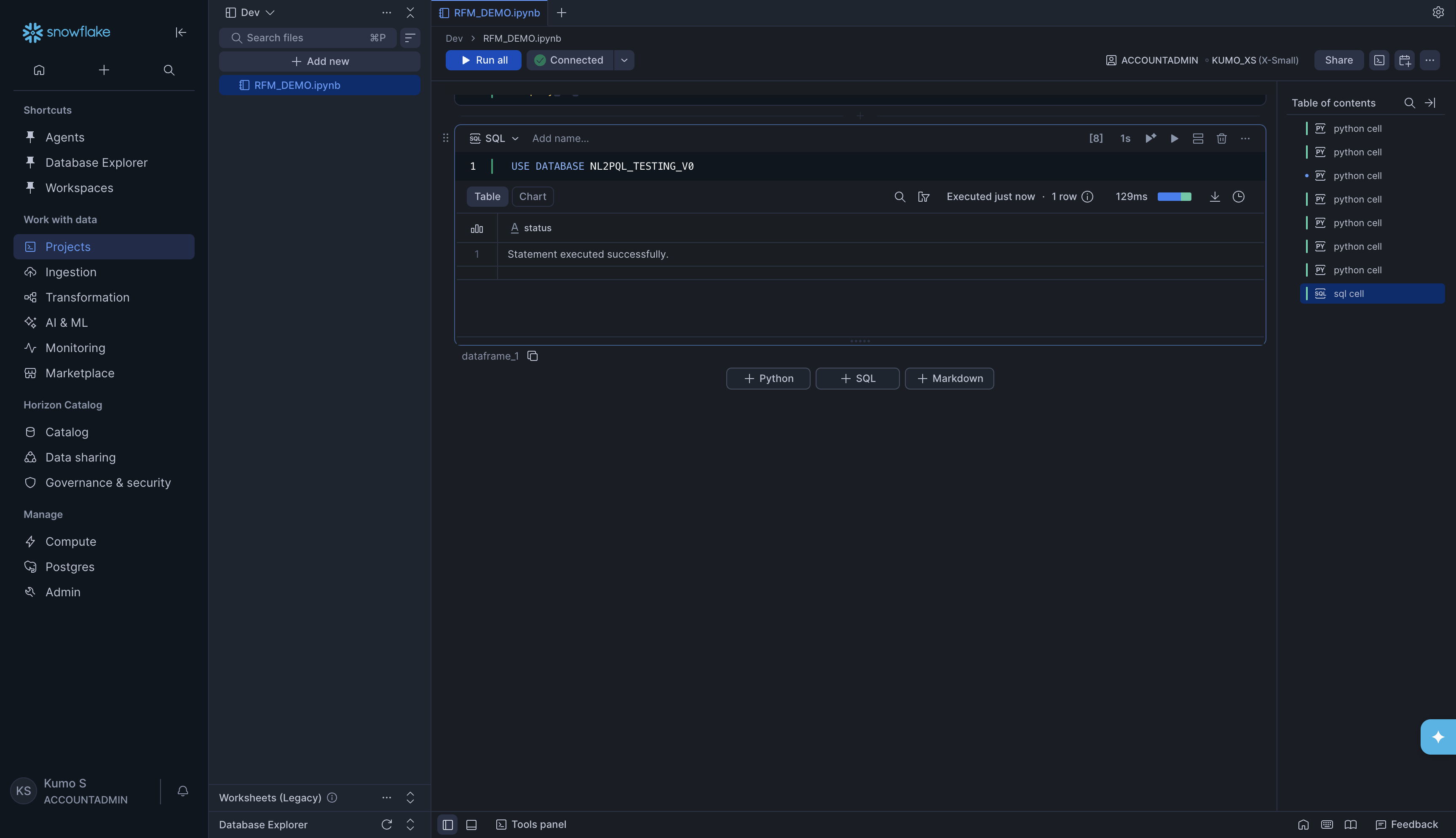
Tip

To add a SQL cell, click + SQL at the bottom of the notebook.

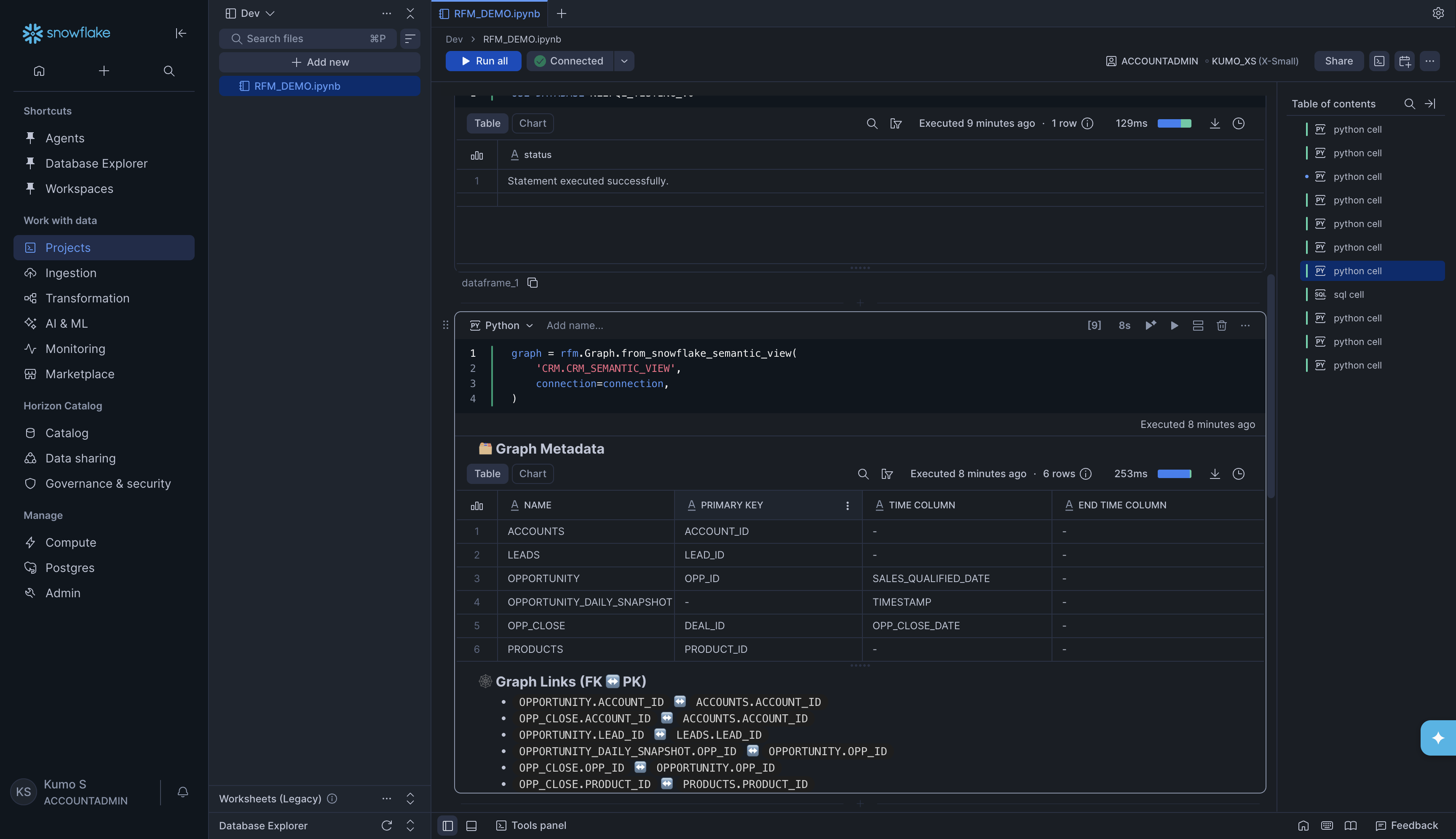
Build the graph from the semantic view:

graph = rfm.Graph.from_snowflake_semantic_view(
    'CRM.CRM_SEMANTIC_VIEW',
    connection=connection,
)

KumoRFM will read the semantic view and discover all tables, columns, and relationships automatically. You will see the Graph Metadata table and Graph Links printed as output.

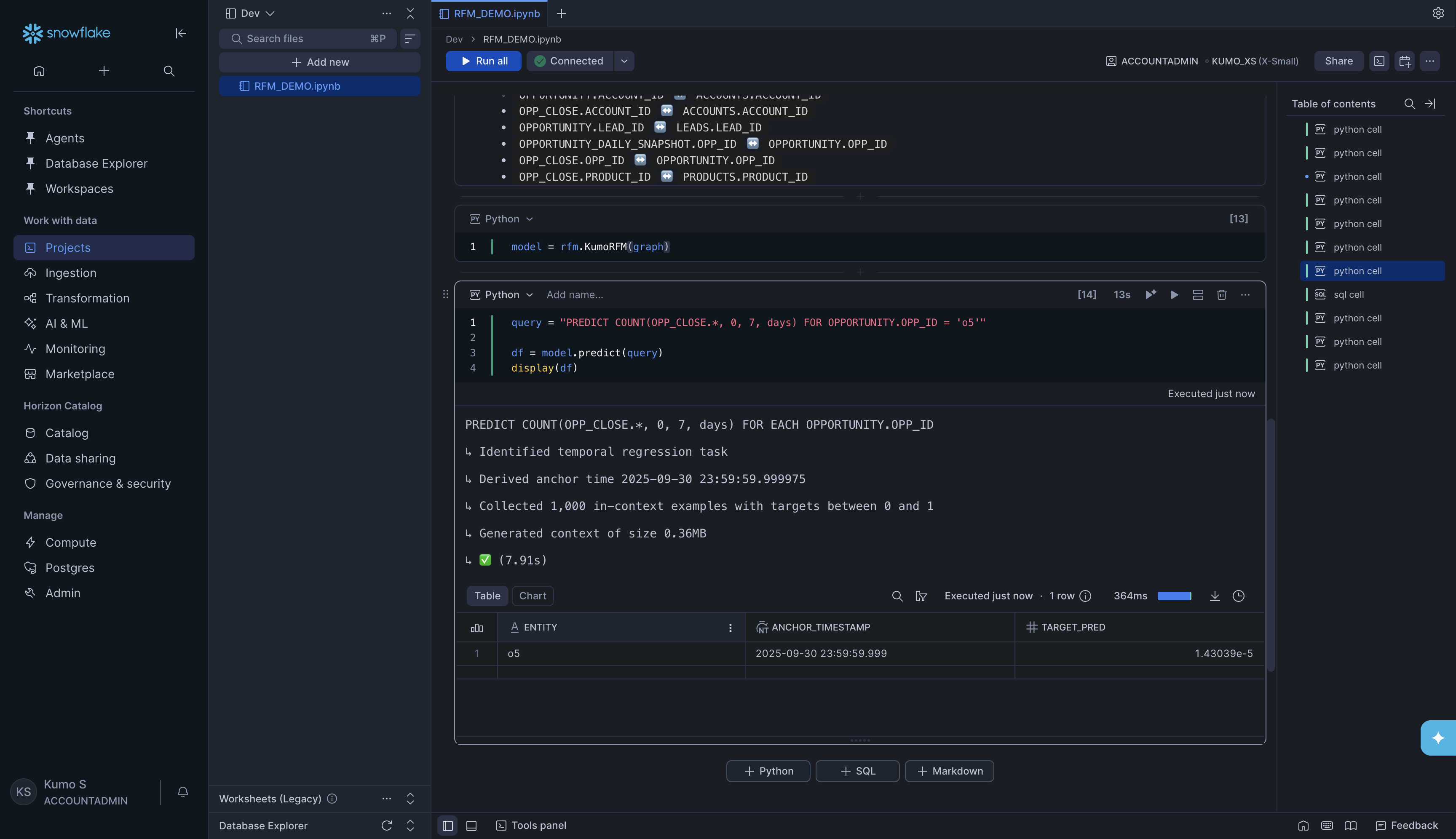
Graph from Semantic View with metadata output

Load the graph and run a prediction:

model = rfm.KumoRFM(graph)

query = "PREDICT COUNT(OPP_CLOSE.*, 0, 7, days) FOR OPPORTUNITY.OPP_ID = 'o5'"

df = model.predict(query)
display(df)

Option C: From Snowflake tables directly#

For production use, you will typically point KumoRFM at your Snowflake tables directly. You create a SnowTable for each table, then combine them into a Graph.

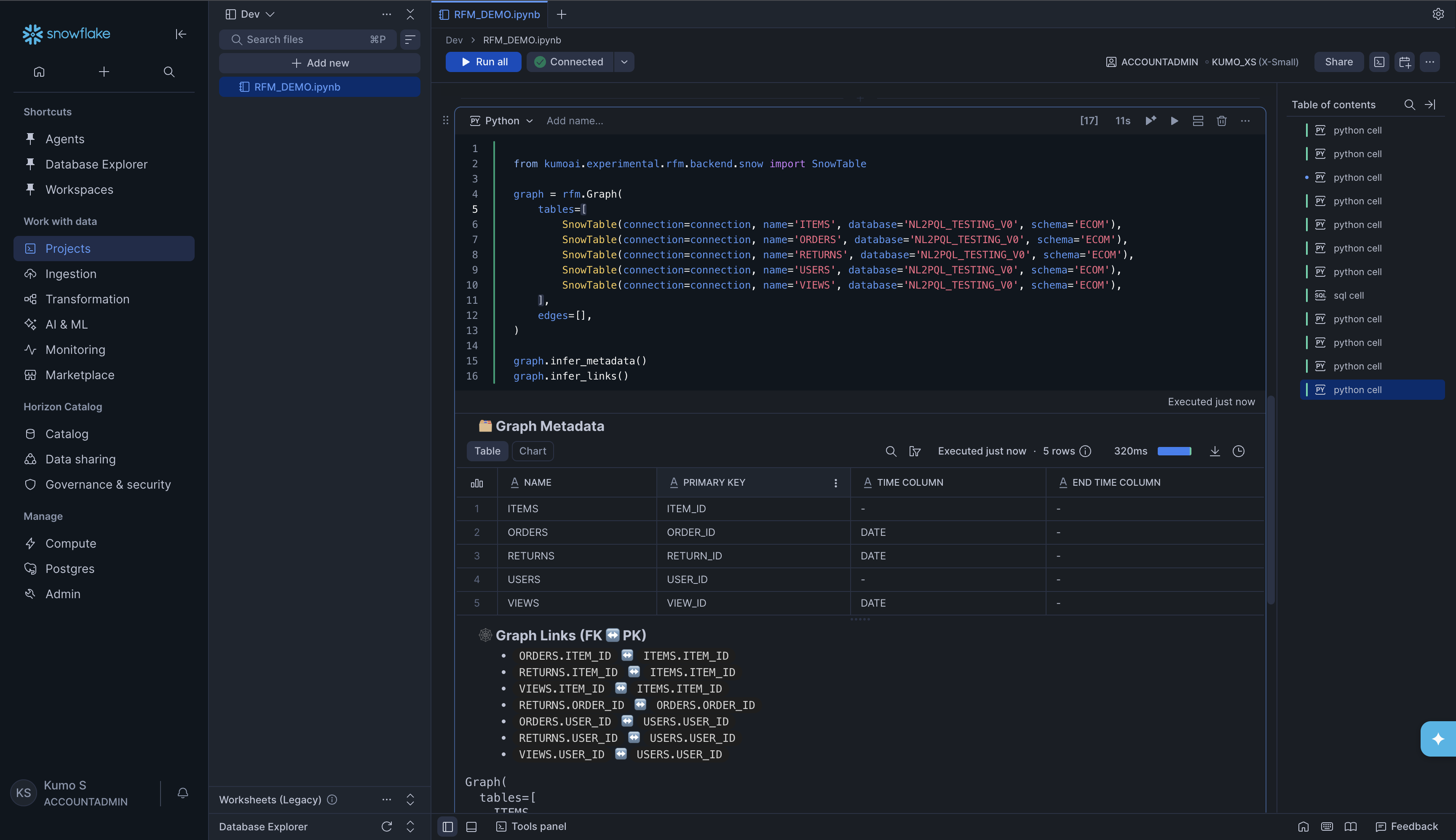
Build the graph from Snowflake tables:

from kumoai.rfm.backend.snow import SnowTable

graph = rfm.Graph(
    tables=[
        SnowTable(connection=connection, name='ITEMS', database='NL2PQL_TESTING_V0', schema='ECOM'),
        SnowTable(connection=connection, name='ORDERS', database='NL2PQL_TESTING_V0', schema='ECOM'),
        SnowTable(connection=connection, name='RETURNS', database='NL2PQL_TESTING_V0', schema='ECOM'),
        SnowTable(connection=connection, name='USERS', database='NL2PQL_TESTING_V0', schema='ECOM'),
        SnowTable(connection=connection, name='VIEWS', database='NL2PQL_TESTING_V0', schema='ECOM'),
    ],
    edges=[],
)

graph.infer_metadata()
graph.infer_links()

Replace the database, schema, and table name values with your own. KumoRFM will detect primary keys, time columns, and foreign key relationships automatically.

SnowTable graph creation with metadata output

Load the graph and run a prediction:

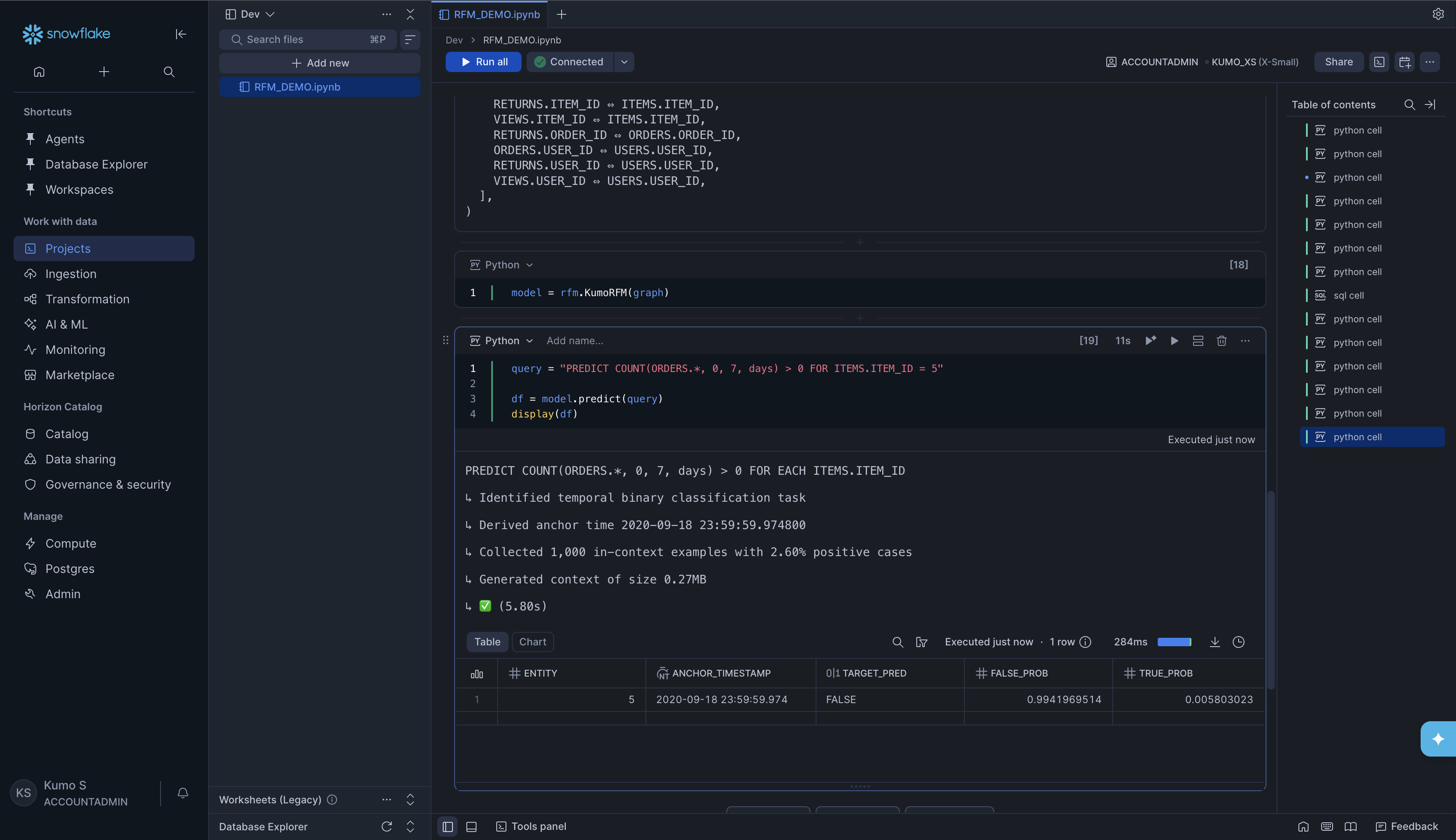
model = rfm.KumoRFM(graph)

query = "PREDICT COUNT(ORDERS.*, 0, 7, days) > 0 FOR ITEMS.ITEM_ID = 5"

df = model.predict(query)
display(df)

Understanding the Prediction Output#

Regardless of which option you used above, the prediction result is always a pandas DataFrame. The columns depend on the type of prediction:

Column	Description
`ENTITY`	The entity you predicted for (e.g., a user ID, item ID, or opportunity ID)
`ANCHOR_TIMESTAMP`	The point in time the prediction is made from. By default, this is the latest timestamp in your data.
`TARGET_PRED`	The predicted value or class
`FALSE_PROB` / `TRUE_PROB`	For binary classification tasks only -the probability of each outcome

What’s Next#

Querying KumoRFM -Learn PQL syntax in detail
Supported Prediction Types -All supported prediction types (classification, regression, forecasting, and more)
Filters and Operators -Filter and refine your queries
Evaluation -Evaluate prediction quality
Configuration -Run modes, explainability, batch predictions
Snowflake Connector -More details on Snowflake table configuration

KumoRFM in Snowflake Notebooks

Contents

KumoRFM in Snowflake Notebooks#

Setup#

Step 1. Open Snowflake and go to Workspaces#

Step 2. Create a new Notebook#

Step 3. Connect your Notebook#

Step 4. Install the Kumo SDK#

Step 5. Import and initialize#

Build Your Graph and Make Predictions#

Option A: From pandas DataFrames (LocalGraph)#

Option B: From a Snowflake Semantic View#

Option C: From Snowflake tables directly#

Understanding the Prediction Output#

What’s Next#